BERT: Bidirectional Encoder Representations from Transformers#

The year 2018 marked a turning point for the field of Natural Language Processing (NLP).
The BERT [Devlin et al., 2018] paper introduced a new language representation model that outperformed all previous models on a wide range of NLP tasks.
BERT is a deep bidirectional transformer model that is pre-trained on a large corpus of unlabeled text.
The model is trained to predict masked words in a sentence and is also trained to predict the next sentence in a sequence of sentences.
The pre-trained model can then be fine-tuned on a variety of downstream NLP tasks with state-of-the-art results.
BERT builds on two key ideas:
The transformer architecture [Vaswani et al., 2017]
Unsupervised pre-training
BERT is pre-trained on a large corpus of unlabeled text. Its weights are learned by predicting masked words in a sentence and predicting the next sentence in a sequence of sentences.
BERT is a deep bidirectional transformer model. It is a multi-headed beast with 12(24) layers, 12(16) attention heads, and 110 million parameters. Since model weights are not shared across layers, the total number of different attention weights is 12(24) x 12(16) = 144(384).
The Architecture of BERT#
The core component of BERT is the attention mechanism.
Attention is a way for a model to assign weights to different parts of the input based on their importance to some task.
For the sentence The dog from down the street ran up to me and ___, to complete the sentence, a model may give more attention to the word dog than to the word street. Because knowing that the subject of the sentence is a dog is more important than knowing that where the dog is from.
Attention Mechanism#
The attention mechanism is quite simple. It is a function that takes in two inputs: a query and a key. The query is the part of the input that we want to focus on. The key is the part of the input that we want to compare the query to. The output of the attention mechanism is a weighted sum of the values of the key. The weights are computed by a function of the query and the key.
Suppose you have some sequence of words \(X\), where each element \(x_i\) is a (refered to as the value) of dimension \(d\).
In the following example, \(X\) is a sequence of 3 words, each represented by a 4-dimensional vector.

Attention is simply a function that takes X as input and returns another sequence Y of the same length as X, composed of vectors of the same dimension as the vectors in X.
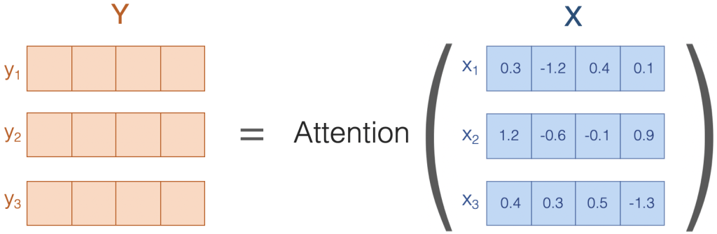
Each vector in Y is computed by taking a weighted average of the vectors in X.

That is, attention is just a weighted average of the values of the vectors in X. The weights show how much the model attends to each vector in X when computing the output vector.
Attending to language#
How does attention work in the context of language?
Suppose we have a sentence the dog ran. We can represent this sentence as a sequence of vectors, where each vector is a word embedding.

A word embedding is a vector representation of a word. It is a vector of real numbers. Each element of the vector represents a dimension of the word that captures some aspect of its meaning.
Those aspects can be semantic, syntactic, or even phonetic. For example, the first element of the vector may represent the semantic meaning of the word, the second element may represent the syntactic meaning of the word, and the third element may represent the phonetic meaning of the word.
In practice, word embeddings are not interpretable. We don’t know what each element of the vector represents. But we can use them to compute the meaning of a sentence.
For example, we can perform arithmetic operations on word embeddings. For example, we can compute the vector representation of the word cat by adding the vectors of the words kitten and dog and subtracting the vector of the word puppy.
Attention is also a form of arithmetic operation. Therefore, you can apply attention to word embeddings to compute the meaning of a sentence.
For example, the embedding of the word dog in \(Y\) is computed by taking a weighted average of the embeddings of the words the, dog, and ran in \(X\) with weights of 0.2, 0.7, and 0.1 respectively.
How does this process help the model to understand the meaning of a sentence?
To fully understand the meaning of a sentence, we need to know the meaning of each word in the sentence. But we can’t just look at each word in the sentence in isolation. We need to know the context of the word.
The attention mechanism allows the model to focus on the words that are most important to the meaning of the sentence.
Multi-head attention#
BERT learns multiple attention mechanisms, called heads, which operate in parallel. Each head is a different attention mechanism. The output of each head is concatenated and fed into a feed-forward neural network.
Multi-head attention enables the model to learn broader types of relationships between words in a sentence than a single attention mechanism.
BERT also stacks multiple layers of multi-head attention. Each layer of multi-head attention takes the output of the previous layer as input. The output of the last layer of multi-head attention is fed into a feed-forward neural network.
Through this architecture, BERT is able to learn very rich representations of language as it gets to the deeper layers of the network.
Because the attention heads do not share parameters, each head learns a different type of relationship between words in a sentence.
Visualizing Attention#
# %pip install bertviz
%config InlineBackend.figure_format='retina'
from bertviz import model_view, head_view
from bertviz.neuron_view import show
from transformers import AutoTokenizer, AutoModel, utils
utils.logging.set_verbosity_error() # Suppress standard warnings
model_version = "bert-base-uncased"
tokenizer = AutoTokenizer.from_pretrained(model_version)
model = AutoModel.from_pretrained(model_version, output_attentions=True)
sentence_a = "I went to the store."
sentence_b = "At the store, I bought fresh strawberries."
inputs = tokenizer.encode(
[sentence_a, sentence_b],
return_tensors="pt",
)
outputs = model(inputs)
attention = outputs[-1]
tokens = tokenizer.convert_ids_to_tokens(inputs[0])
Each cell in the model view shows the attention pattern of a single head. The attention pattern of each head is different. The attention patterns are specific to the input sentence.
# model_view(attention, tokens)
Deconstructing Attention#
Let’s take a closer look at how attention works.
Now that we know that attention is a weighted average of the values of the vectors in X, let’s look at how the weights are computed.
The weights are computed by a function of the query and the key. The query is the part of the input that we want to focus on. The key is the part of the input that we want to compare the query to.
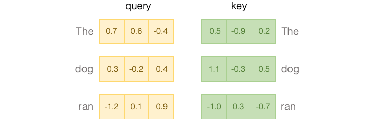
These vectors can be thought of as a type of word embedding like the value vectors we saw earlier, but constructed specifically for determining the similarity between words.
The similarity between two words is computed by taking the dot product of the query and key vectors of those words.

To convert the dot product into a probability, we apply a softmax function to the dot product, which normalizes the dot product so that it sums to 1.
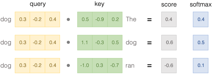
The softmax values on the right represent the final weights of the attention mechanism.
Where do these query and key vectors come from?#
We now understand that attention weights are computed from query and key vectors. But where do these vectors come from?
The query and key vectors are computed from the value vectors. The query and key vectors are computed by passing the value vectors through two different linear layers.
We can visualize how attention weights are computed from query and key vectors using the neuron view.
This view traces the computation of attention from the selected word on the left to the complete sequence of words on the right. Positive values are colored blue and negative values orange, with color intensity representing magnitude.
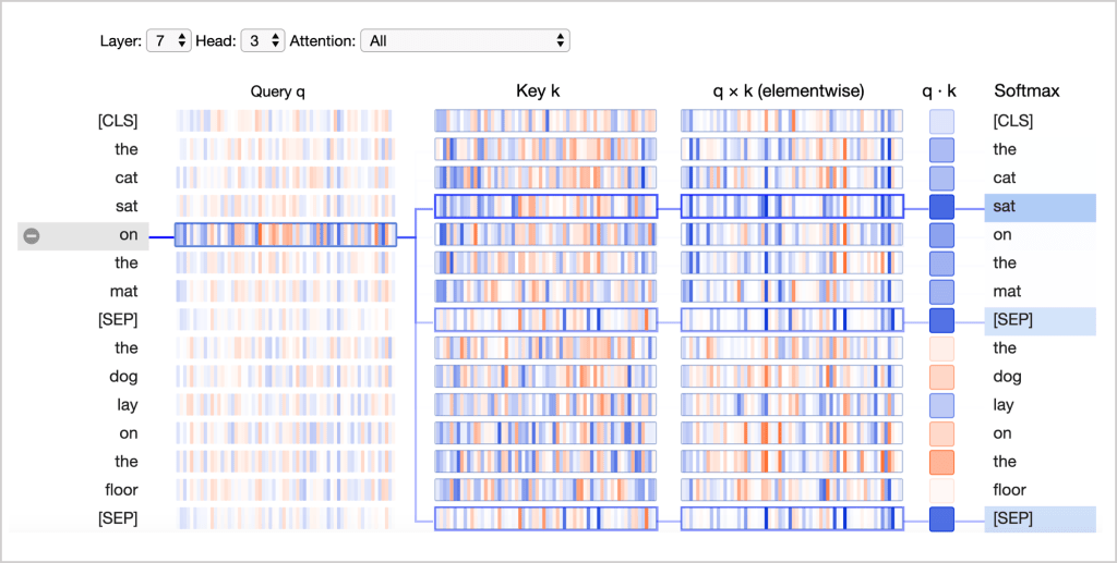
Let’s go through the columns in the neuron view one at a time.
Query q: the query vector q encodes the word on the left that is paying attention, i.e. the one that is “querying” the other words. In the example above, the query vector for “on” (the selected word) is highlighted.
Key k: the key vector k encodes the word on the right to which attention is being paid. The key vector and the query vector together determine a compatibility score between the two words.
q×k (elementwise): the elementwise product between the query vector of the selected word and each of the key vectors. This is a precursor to the dot product (the sum of the elementwise product) and is included for visualization purposes because it shows how individual elements in the query and key vectors contribute to the dot product.
q·k: the scaled dot product (see above) of the selected query vector and each of the key vectors. This is the unnormalized attention score.
Softmax: the softmax of the scaled dot product. This normalizes the attention scores to be positive and sum to one.
Explaining BERT’s attention patterns#
Let’s explore the attention patterns of various layers of the BERT (the BERT-Base, uncased version).
Sentence A: I went to the store.
Sentence B: At the store, I bought fresh strawberries.
BERT uses WordPiece tokenization and inserts special classifier ([CLS]) and separator ([SEP]) tokens, so the actual input sequence is:
[CLS] I went to the store . [SEP] At the store , I bought fresh straw ##berries . [SEP]
from bertviz.transformers_neuron_view import BertModel, BertTokenizer
from bertviz.neuron_view import show
model_type = 'bert'
do_lower_case = True
neuron_model = BertModel.from_pretrained(model_version, output_attentions=True)
neuron_tokenizer = BertTokenizer.from_pretrained(model_version, do_lower_case=do_lower_case)
show(neuron_model, model_type, neuron_tokenizer, sentence_a, sentence_b, layer=2, head=0)